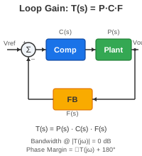
A regulator compares what you want (\(V_\text{ref}\)) to what you have (\(V_\text{out}\)) and drives the error toward zero. Without feedback, the output drifts with load, line, and temperature. With feedback, the loop forces \(V_\text{out} \to V_\text{ref}\) — but only if the loop is stable.
You already know how to write \(H(s)\) for a single block (see the Transfer Function Primer). A power-supply control loop is several such blocks wired in a circle. This page stays abstract: no circuits, only transfer functions.
Every classical loop has the same skeleton: a reference, a summer, a forward path, and a return path.
The error signal at the summer is:
\[ e(s) = V_\text{ref}(s) - F(s)\,V_\text{out}(s) \]Plant \(P(s)\) is the power stage and output filter. Compensator \(C(s)\) shapes the loop. Feedback \(F(s)\) is usually a resistor divider — often just a constant gain. We draw boxes, not schematics.
Trace the algebra in three steps. The forward chain from error to output is \(L(s) = C(s)\,P(s)\):
\[ V_\text{out}(s) = L(s)\,e(s) \] \[ e(s) = V_\text{ref}(s) - F(s)\,V_\text{out}(s) \]Substitute and solve for \(V_\text{out}/V_\text{ref}\):
\[ T_\text{cl}(s) = \frac{V_\text{out}(s)}{V_\text{ref}(s)} = \frac{L(s)}{1 + L(s)\,F(s)} \]
When the denominator goes to zero, the loop blows up.
Instability means closed-loop poles where
In plain language: at some frequency the loop has unity gain and −180° phase — the returned signal reinforces the error instead of canceling it.
2nd-order approximation from BW and PM — same engine as the transient panel below.
To analyze stability we break the loop at the summer: inject a test signal and ask what comes back around. The open-loop transfer function — usually called loop gain — is the product of every block in the circle:
\[ T(s) = P(s)\,C(s)\,F(s) \]On a Bode plot we draw \(|T(j\omega)|\) in dB and \(\angle T(j\omega)\) in degrees. Loop gain is not the same as the closed-loop response \(T_\text{cl}(s)\) — it is what we measure and shape during design.
Loop bandwidth \(f_\text{bw}\) is the frequency where the loop gain crosses unity:
\[ |T(j\omega_\text{bw})| = 1 \quad (0\,\text{dB}) \]Below \(f_\text{bw}\) the loop has gain and rejects load and line disturbances. Above \(f_\text{bw}\) the loop cannot correct fast enough. Higher bandwidth generally means faster response — but only if phase margin stays healthy.
Phase margin (PM) is the phase headroom at the 0 dB crossing — how far \(\angle T(j\omega)\) sits above the −180° stability line:
\[ \text{PM} = 180° + \angle T(j\omega_\text{bw}) \]Example: if \(\angle T = -120°\) at crossover, then PM \(= 180° + (-120°) = 60°\). At −180° exactly, the loop would oscillate.
Plant \(P(s)=1/(1+s/\omega_p)\), Type-II compensator \(C(s)=(1+s/\omega_z)/[s(1+s/\omega_c)]\), unity feedback. Pick PM, slide bandwidth — \(K\) and pole/zero locations are solved behind the scenes. Green ○ = zero, red × = pole (origin pole at left edge).
PM is a frequency-domain number — but it shows up as how the output recovers from a unit load step. Fixed axes (Bode to 1 MHz, step to 5 ms) so traces slide as you change BW and PM.
Green ○ = zero, red × = pole (origin pole at left edge of plot). Full-featured version: Control System Transient Analyzer
Holding PM fixed, a wider loop bandwidth means the loop corrects faster — shorter rise and settling time. Push bandwidth up without adding phase (e.g. with a compensator zero), and PM falls — ringing returns.
\[ \zeta \approx \frac{\text{PM}}{100} \quad\text{(rule of thumb)} \] \[ t_s \approx \frac{4}{\zeta\,\omega_n} \]These links are approximate. Bode analysis gets you close; confirm with a load step in simulation or on the bench. Try BW and PM yourself in the Transient Analyzer.
The plant \(P(s)\) is usually low-pass — it eats phase before crossover. Feedback \(F(s)\) is often a constant divider. The compensator \(C(s)\) exists to buy phase back: a zero below crossover, a pole above. That is why power supplies use Type II or Type III networks — not magic, just pole-zero placement on \(T(s)\).
Shape \(P\), \(C\), and \(F\) live in the Feedback Network Analyzer or Type II Compensator tool.
Bode analysis is fast and indispensable, but it focuses on one frequency (crossover) and assumes linear, small-signal behavior. It does not show saturation, slew limits, or large-signal effects.
Root locus complements Bode: instead of magnitude and phase vs frequency, it shows where closed-loop poles move in the \(s\)-plane as gain \(K\) changes. Those poles set oscillation frequency, damping, and settling — directly in the time domain.
Many engineers use Bode to pick a compensator, then root locus to verify the closed-loop poles landed where they expected.