Feedback Network Analyzer

Understanding Loop Gain

Using Bode plots
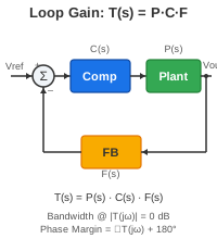
A Bode plot shows how each pole and zero contributes magnitude (dB) and phase (degrees) versus frequency. In this tool, loop gain is P + C + F in dB — the open-loop product split into plant, compensator, and feedback. Hover any chart to sync crosshairs at the same frequency. The gray line marks loop bandwidth (0 dB crossover). The @BW readouts show each block's contribution there.

Phase margin — convention and tips
In most textbooks, phase margin is the distance from −180° at crossover — the stability line for negative feedback, which already implies a −180° inversion around the loop. You read how much phase "headroom" remains above that line (e.g. 60° margin means loop phase is −120° at crossover).

The loop-gain chart defaults to the standard textbook view: phase is P + C + F with the −180° stability line on the plot. Use Folded (−360° view) to include the feedback inversion in the trace (axis −360° to −180°) — same phase margin, different bookkeeping. The loop-math readout matches whichever view is selected.

Practical targets:

• 45–60° — common for power-supply loops; stable without being sluggish
• Below ~30° — expect ringing or bench instability
• Very high PM — often a low crossover; transients may be slow

Wider bandwidth usually means faster correction but less phase. Pushing crossover up almost always requires phase boost (e.g. a compensator zero below crossover).

Why Bode isn't the whole story
Bode analysis is fast for compensation, but it focuses on crossover and uses approximations (phase margin ↔ damping is a rule of thumb, not exact). It assumes linear behavior — large-signal limits and saturation won't show up. Layout parasitics and filter poles still count; leave margin beyond the ideal plot. Use Bode to get close, then confirm with a load step in simulation or on the bench.