PID Pole-Zero Bridge
Two languages for the same compensator
The familiar picture is a parallel PID: proportional, integral, and derivative branches each process the error and sum to the control voltage \(v_c\). Your firmware wants the coefficients \(K_p\) and \(K_i\).
For the vast majority of power converters, the designer does not tune \(k_d\), \(k_p\), and \(k_i\) directly. Rather, the designer positions zeros and poles in the compensator transfer function to meet crossover frequency and phase margin.
Same compensator, two vocabularies. This lesson builds the bridge for PI and optional D: scroll through each branch, watch the Bode plots, read off firmware coefficients. Compare the passive-network view in the Type II Compensator lesson when you are ready.
Vocabulary: Pole/Zero Primer · Classical Feedback
§1 — Parallel PID form (Fig 1.13)
Figure 1.13 shows the parallel form: three branches driven by the same error \(\varepsilon(t)\), summed into \(v_c(t)\):
\[ v_c(t) = k_p\,\varepsilon(t) + k_i\int_0^t \varepsilon(\tau)\,d\tau + k_d\frac{d\varepsilon}{dt} \]In the Laplace domain (PI core; D optional with a filter pole):
\[ C(s) = K_p + \frac{K_i}{s} + \frac{K_d s}{1 + s/\omega_f} \]Factored the way you already think about Type II:
\[ C(s) = K_p \cdot \frac{1 + s/\omega_z}{s}, \quad \omega_z = \frac{K_i}{K_p} \]The integrator \(1/s\) is a pole at the origin. The zero sits at \(\omega_z = K_i/K_p\). In Hz: \(f_z = K_i/(2\pi K_p)\).
Dig deeper — standard form (Fig 4.1)
Textbooks also show an equivalent standard form where time constants \(\tau_i\), \(\tau_d\) sit inside the blocks and \(k_p\) scales the sum:
\[ v_c = k_p\left[\varepsilon + \frac{1}{\tau_i}\int\varepsilon\,dt + \tau_d\frac{d\varepsilon}{dt}\right] \]Expanding gives the parallel form above, with \(k_i = k_p/\tau_i\) and \(k_d = k_p\tau_d\). We use the parallel form throughout because those are the values you load into firmware.
Pole / zero map
P
\[ C_p(s) = K_p \]Scalar gain — no finite poles or zeros.
I
\[ C_i(s) = \frac{K_i}{s} = K_p\,\frac{1 + s/\omega_z}{s}, \quad \omega_z = \frac{K_i}{K_p} \] \[ \text{pole: } s = 0 \qquad \text{zero: } \omega_z \qquad f_z = \frac{K_i}{2\pi K_p} \]Here the breakpoint \(f_z\) is the zero — same frequency.
D
\[ C_d(s) = \frac{K_d s}{1 + s/\omega_f} \] \[ \text{zero: } s = 0 \qquad f_d = \frac{K_p}{2\pi K_d} \qquad f_\text{safety} = N f_d \]Zero at \(s=0\): the numerator is \(K_d s\), so magnitude rises at +20 dB/dec from the origin — that is the zero doing its job.
\(f_d\) is not that zero. It is where \(|K_d j\omega|\) crosses \(K_p\) on the Bode plot — the frequency where the D-branch level equals P, the same idea as \(f_z\) for I but without being a pole or zero location.
\(f_\text{safety}\): real pole from the noise filter (\(\omega_f = 2\pi f_\text{safety}\)), typically \(N=5\) above \(f_d\).
§2 — P is just gain
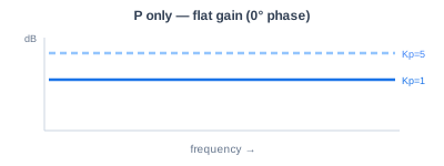
Before adding dynamics, \(K_p\) alone is flat magnitude and 0° phase in the mid band. In pole-zero language it is the scalar K in dB out front — no poles or zeros yet.
The Bode plot shows magnitude in dB. \(K_p\) is a voltage gain (linear ratio of error to control contribution), so:
\[ K_{\text{dB}} = 20\log_{10}(K_p) \]Use 20 log for voltage or current amplitude ratios — power scales as amplitude squared, so power ratios use 10 log. At \(K_p = 1\), the trace sits at 0 dB. \(K_p\) is floored at 0.1 here so the gain line stays visible on the plot.
§3 — Integrator I adds a pole at the origin
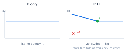
The I branch is \(K_i/s\) — an integrator. That is a pole at \(s = 0\): −20 dB/decade and −90° phase lag at low frequency, which is what drives steady-state error to zero in the closed loop.
Note: \(f_i = K_i/(2\pi K_p)\) is where the integrator magnitude equals \(K_p\) — it is not a pole. The pole sits at the origin.
§4 — Tuning console (the bridge)
Set the plant first, then shape the compensator, and read the loop gain at the bottom. The Type II zero at \(f_z\) is the same as \(K_i\): \(\omega_z = K_i/K_p\). Note \(f_i = f_z\) — where the I-term magnitude equals \(K_p\); it is not a pole.
Plant \(P(s)\)
First order: \(P(s) = K_\text{plant}/(1 + s/\omega_p)\), pole at \(f_p = \omega_p/(2\pi)\). Second order adds \(f_{p2}\).
Compensator \(C(s)\)
Poles and zeros from the parallel form:
\[ f_z = f_i = \frac{K_i}{2\pi K_p}, \quad \text{origin pole from } \frac{K_i}{s} \] \[ f_d = \frac{K_p}{2\pi K_d}, \quad f_\text{safety} = N\,f_d \;\;(N=5\;\text{default}) \]Pole / zero inventory
Transfer functions
§5 — Plant and loop (precision vs stability)
Every loop trades precision against stability. Start with the plant plot — that is the raw dynamics you cannot change without hardware. The loop-gain plot is \(T(s)=C(s)P(s)\) (unity feedback): crossover and phase margin live there. Place \(f_z\) below \(f_p\) to start. A second-order plant often needs D for extra phase lead.
Compare the passive network view in the Type II Compensator lesson when you are ready.
References
- Christophe Basso, Designing Control Loops for Linear and Switching Power Supplies: A Tutorial Guide (Artech House) — §1.3.5 (Fig 1.13, parallel PID), §4.1 (standard vs parallel form, filtered D), §4.1.3 (PI), §4.2.8 (Type 2a), §4.2.10 (Type 3 / double zero).